Lecture 9 - Tuning

Last updated Mar 24, 2023

Slides

• Faster = higher throughput, or lower response time
• Avoid bottlenecks
• 5% is a lot

• Troubleshooting
• Capacity Sizing
• Application Programming

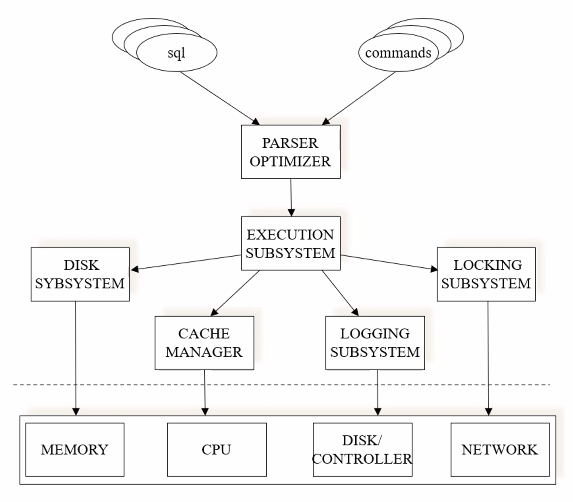
Causes of bad performance may have to do with disk size, log system, locks…

1. Think globally, fix locally
   • we have to know everything about the DB to investigate what is going on
   • usually the solution is a simple change
2. . Partitioning breaks bottlenecks
   • temporal and spatial
   • many transaction may compete for the same resources
3. Start-up costs are high; running costs are low
   • bringing data to memory is costly (finding execution plans)
4. Render unto server what is due unto server
   • take the most advantage of the DB system (joins, logic operations…)
5. Be prepared for trade-offs
   • indexes are trade-offs (inserting data means updating indexes)

• Schema tuning
• Query Tuning

consists of changinf the tables of the database to get better perfiormance

A relation R is normalized if every interesting functional dependency X -> A has the property that X is a key of R

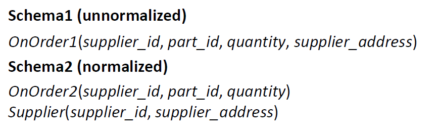
• OnOrder1 is not normalized, because the key is ( supplier_id , part_id ) but supplier_id alone determines supplier_address
• OnOrder2 and Supplier are normalized

Normalization is not always better

• Space: Schema 2 saves space, we are not repeating the supplier_address

• Update anomalies (information preservation): Some supplier addresses might get lost with schema 1 if a supplier is deleted once the order has been filled

• Performance trade-off: In case of frequent accesses to supplier’s address given an ordered part, then schema 1 is good, specially if there are few updates

Denormalizing means sacrificing normalization for the sake of performance:

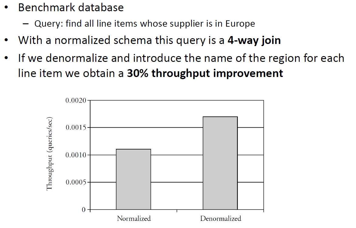
• Denormalization speeds up performance when attributes from different normalized relations are often accessed together
• Denormalization hurts performance for relations that are often updated

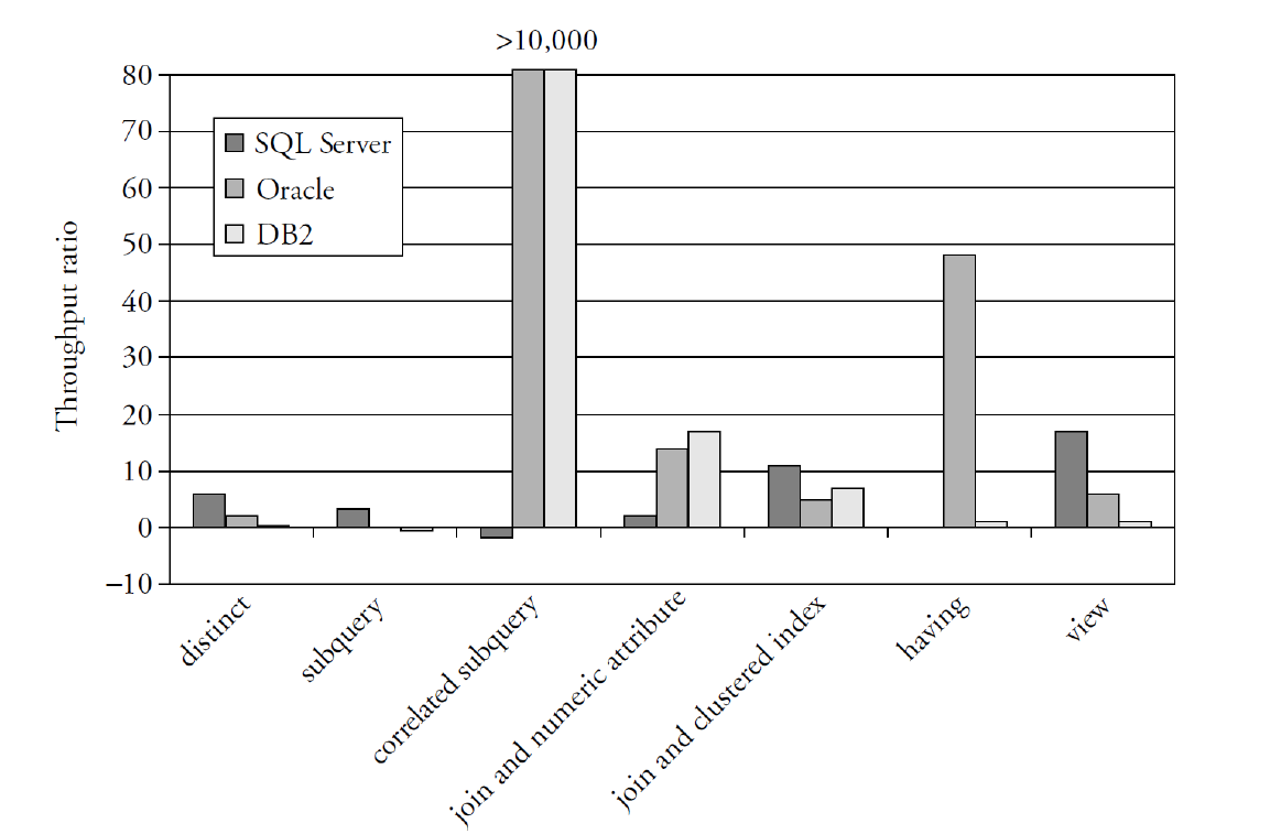
See Slides for Benchmark

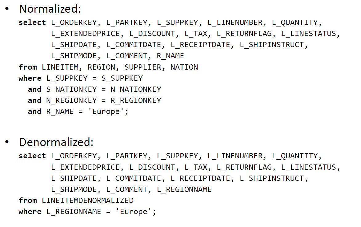
The query: “find all line items whose supplier is in Europe”

In a Normalized schema 600 000 line items, 500 suppliers, 25 nations, 5 regions In a Denormalized one 600 000 line items

Three attributes: account_ID , balance , address

• Functional dependencies:

  • account_ID->balance
  • account_ID->address

• Two possible normalized schema designs: ( account_ID , balance , address ) or ( account_ID , balance ) ( account_ID , address )

Q: Which design is better? R: It depends on the query pattern .

• The address is used mainly by the application that sends a monthly account statement
• The balance is updated or examined several times a day

The second schema might be better because the relation ( account_ID , balance ) can be made smaller

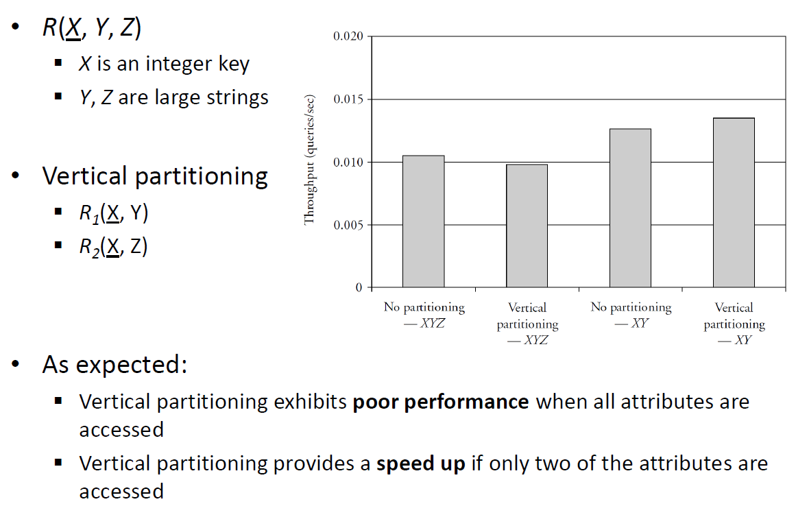
A single normalized relation XYZ is better than two normalized relations XY and XZ for queries accessing X, Y, Z together

The two relation design is better if:

• Accesses to X, Y and X, Z are separate most of the time
• Attributes Y or Z have large values

Benchmarking:

Breaking the rules in the name of performance

The accounting department of a convenience store chain issues queries every 20 minutes to obtain:

• The total dollar amount on order for a particular vendor

• The total dollar amount on order by a particular store

• Original Schema: Orders(ordernum , itemnum , quantity, store, vendor) Item(itemnum , price) Store(store, name)

• The total dollar queries are expensive vendor selection on Orders, join with Item on itemnum , multiply price * quantity, then sum similarly for store, possibly requiring join with Store if selection by name

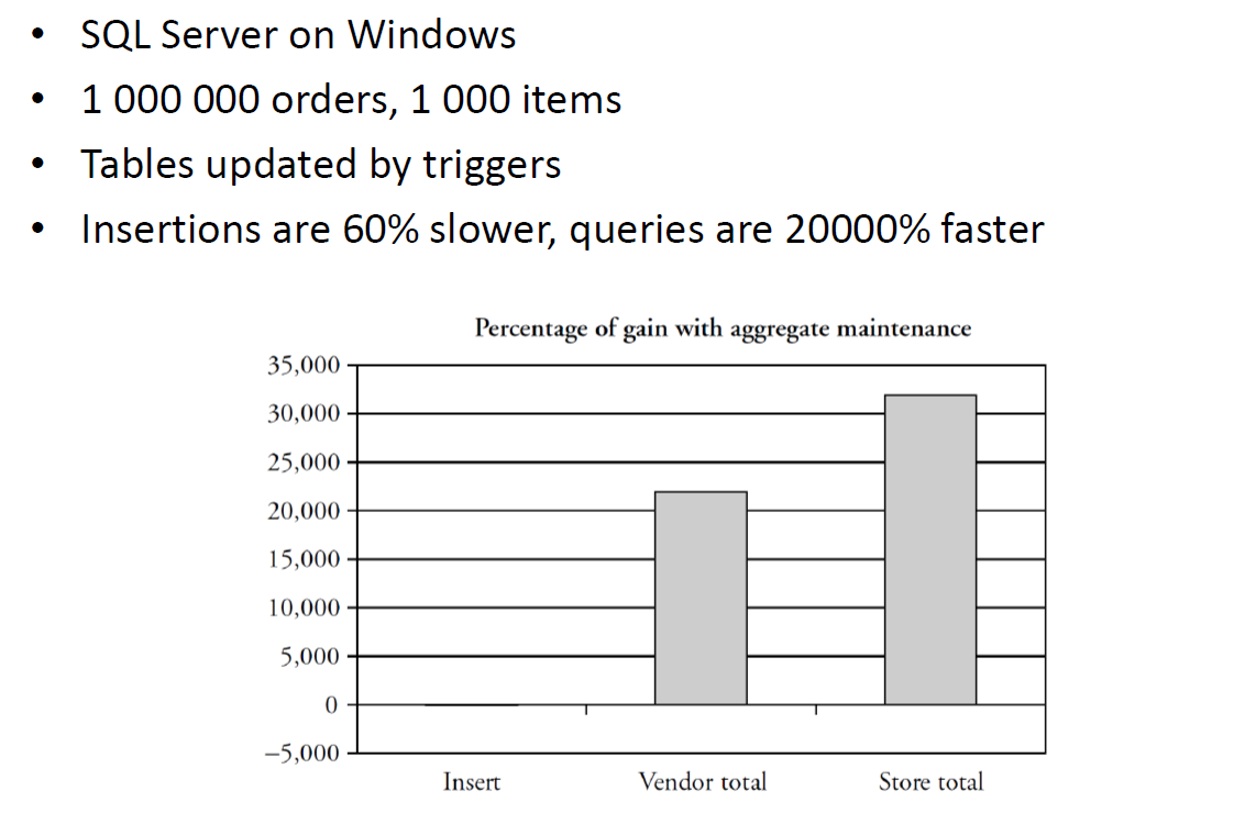
Solution: Aggregation Maintenance

Add the following materialized views:

• VendorTotal (vendor, amount), where amount is the dollar value of goods on order to the vendor, with a clustered index on vendor.

• StoreTotal (store, amount), where amount is the dollar value of goods on order by the store, with a clustered index on store.

• Each update to Orders should update to these two views

  • materialized views take care of these updates implicitly
  • can also be implemented with tables updated by triggers

Benchmark:

• Many query optimizers will not use indexes in the presence of:
  • Arithmetic expressions WHERE salary/12 >= 4000;
  • Substring / upper / lower expressions SELECT * FROM Employee WHERE SUBSTR(name, 1, 1) = ‘G’;
  • Numerical comparisons of fields with different types
  • Comparison with NULL

Ways to eliminate DICTINCT

• sorting
• hashing

PRIMARY KEYs do not repeat

• JOINs on PK do not need DISTINCT

In general, DISTINCT is required when:

• The set of values or records returned should contain no duplicates
• The columns returned do not contain a key of the relation created by the FROM and WHERE clauses

• Call a table T privileged if the fields returned by the SELECT contain a key of T
• Let R be an unprivileged table. Suppose that R is joined on equality by its key field to some other table S , then we say R reaches S
• Now, define reaches to be transitive. So, if R1 reaches R2 and R2 reaches R3 then say that R1 reaches R3

There will be no duplicates among the records returned by a selection, if one of the two following conditions hold:

• Every table mentioned in the FROM clause is privileged
• Every unprivileged table reaches at least one privileged table

See Slides for examples (56~58)

When you use a row from the FROM, you have a nested query See Slides for examples (59~60)

uncorrelated nested queries -> flat query

1. Retain the SELECT clause from the outer block
2. Combine the arguments of the two FROM clauses
3. AND together all the WHERE clauses, replacing IN by =

1
2
3
4

SELECT ssnum
FROM Employee
WHERE dept IN (SELECT dept
FROM Techdept

becomes

1
2
3

SELECT ssnum
FROM Employee, Techdept
WHERE Employee.dept = Techdept.dept

correlated nested queries -> temporary table Query: find the employees who earn more than the average salary in their tech department

1
2
3
4
5
6

SELECT ssnum
FROM Employee e1
WHERE salary > (SELECT avg(e2.salary)
FROM Employee e2, Techdept
WHERE e2.dept = Techdept.dept
AND e2.dept = e1.dept);

This could be inefficient; same average salary computed multiple times

Solution

1
2
3
4
5

INSERT INTO Temp
SELECT avg(salary) as avsalary , Employee.dept
FROM Employee, Techdept
WHERE Employee.dept = Techdept.dept
GROUP BY Employee.dept

Returns the average of salaries per tech department

1
2
3
4

SELECT ssnum
FROM Employee, Temp
WHERE salary > avsalary
AND Employee.dept = Temp.dept

A better solution would be to use a materialized view (automatically created when creating indexes in SQLServer)

Query: Find all employees in the information systems department who earn more than $40000

1
2
3
4
5
6
7
8

INSERT INTO Temp
SELECT *
FROM Employee
WHERE salary > 40000;

SELECT ssnum
FROM Temp
WHERE Temp.dept = 'Information

Optimizer would miss the opportunity to use the index on dept

More efficient solution:

1
2
3
4

SELECT ssnum
FROM Employee
WHERE dept = 'Information Systems'
AND salary > 40000;

Example: Find all students who are also employees

1
2
3

SELECT *
FROM Employee, Student
WHERE Employee.name = Student.name;

Both tables have index on name , but it is a non clustered index;

The following join would be much more efficient:

1
2
3

SELECT *
FROM Employee, Student
WHERE Employee.ssnum = Student.ssnum

Here we can have a MERGE as both tables are sorted on the clustered index on the PK

Do not use HAVING when WHERE is enough

1
2
3
4
5

SELECT avg(salary) as avgsalary , dept
FROM Employee
GROUP BY dept
HAVING dept = 'Information Systems';
SELECT avg(

Here we are creating a GROUP for every dept (bad performance)

1
2
3
4

SELECT avg(salary) as avgsalary , dept
FROM Employee
WHERE dept = 'Information Systems'
GROUP BY dept;

only 1 group!

Views may cause queries to execute inefficiently

1
2
3
4

CREATE VIEW Techlocation AS
SELECT ssnum , Techdept.dept , location
FROM Employee, Techdept
WHERE Employee.dept = Techdept.dept

1
2
3

SELECT dept
FROM Techlocation
WHERE ssnum = 43253265;

The query below will be slower because of the expansion of the view (also price of JOIN) The system might not use the view

Lecture 8 Database Recovery | Lecture 10 Tuning (continued)