Lecture 5 - Query Optimization
# Query Optimization
# Evaluating a given query
Query optimization is finding the optimal execution plan
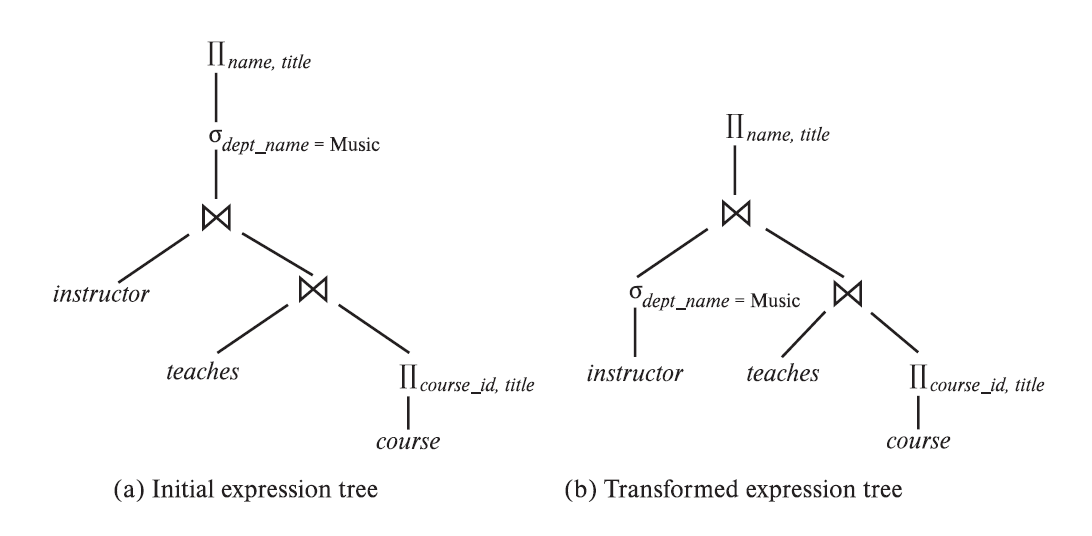
From a) to b) we change the plan because we only join the rows we want, which translates in a better performance becasue has smaller intermediate results
Pushed down selection of rows from a) to b)
We can also push down selection of columns
# Equivalence Rules
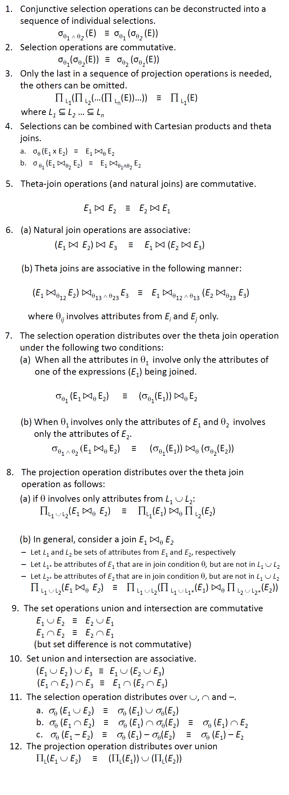
Associative Rules in Joins can be useful to maintain order or use some index
See examples on slides
Performing the selection as early as possible reduces the size of the relation to be joined. Performing the projection as early as possible reduces the size of the relation to be joined.
# Cost-Based Optimization
Now consider finding the best join order for: (r 1 ⨝ r 2 ⨝ r 3 ⨝ r 4 ⨝ r 5)
- There are 12 different join orders for r 1 ⨝ r 2 ⨝ r 3 and another 12 orders for (…) ⨝ r 4 ⨝ r 5 Should we consider 12x12 joins orders?
- No. Only 12+12. We choose the best order for r 1 ⨝ r 2 ⨝ r 3 and the best order for (…) ⨝ r 4 ⨝ r 5 independently.
- When an optimization problem can be solved by optimizing sub problems independently, we can use dynamic programming
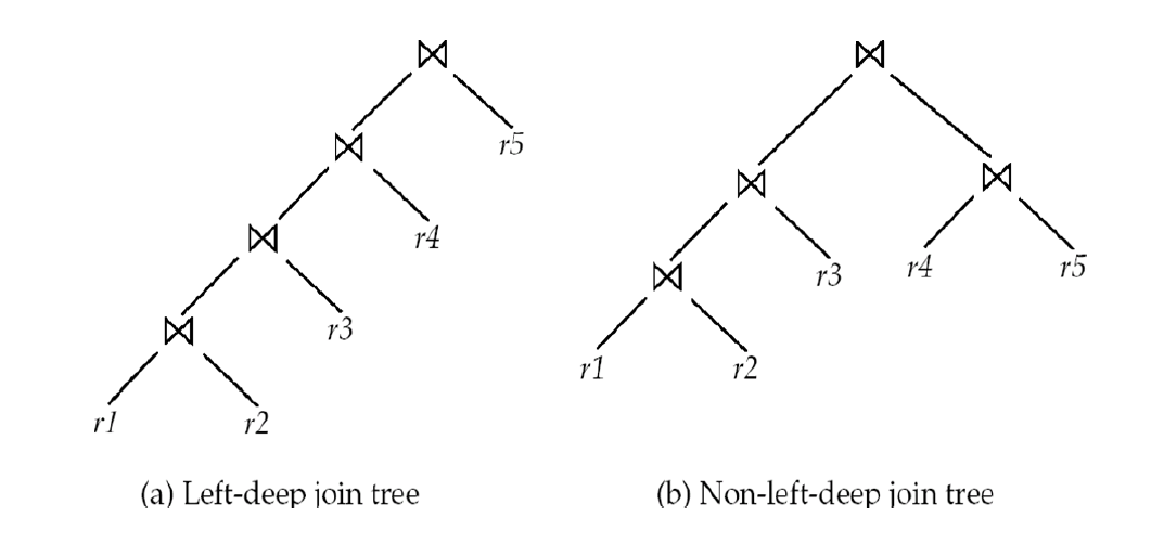
# Heuristics in Optimization
- E.g. in left deep join trees, the right hand side input for each join is always a relation, not the result of an intermediate join.
- Fewer join orders to consider.
# Concept of memoization
- Store the best plan for a subexpression the first time it is optimized, and reuse it on repeated optimization calls on same subexpression
# Implemented as plan caching
- Reuse previously computed plan if query is resubmitted
- Even with different constants in query
- Applies to the exact same query
# Materialized Views
- A materialized view is a view whose contents are computed and stored.
| |
- Materializing the above view would be very useful if the list of students is required frequently
# Query Optimization and Materialized Views
Rewriting queries to use materialized views:
- A materialized view v r ⨝ s is available
- A user submits a query r ⨝ s ⨝ t
- We can rewrite the query as v ⨝ t
Whether to do so depends on cost estimates for the two options The system knows which materialized views exist, so it can use them to optimize the query
Replacing a use of a materialized view:
- A materialized view v r ⨝ s is available
- User submits a query (select)(A =10)(v) but the view has no index on A
- Suppose r has an index on A , and s has an index on the common attribute
- Then the best plan may be to replace v by r ⨝ s, which can lead to the query plan (select)(A =10) r ⨝ s
Query optimizer should consider all above options and choose the best overall plan
# Materialized View Creation
- Materialized view creation : “W hat is the best set of views to materialize?”
- Index creation :“What is the best set of indices to closely related, but simpler
- Materialized view creation and index creation based on typical system workload (queries and
- Typical goal: minimize time to execute workload , subject to constraints on space and time taken for some critical queries/updates
- One of the steps in database tuning (more on tuning in next lectures)
- Commercial database systems provide tools (called " tuning assistants” or “wizards”) to help the database administrator choose what indices and materialized views to create.
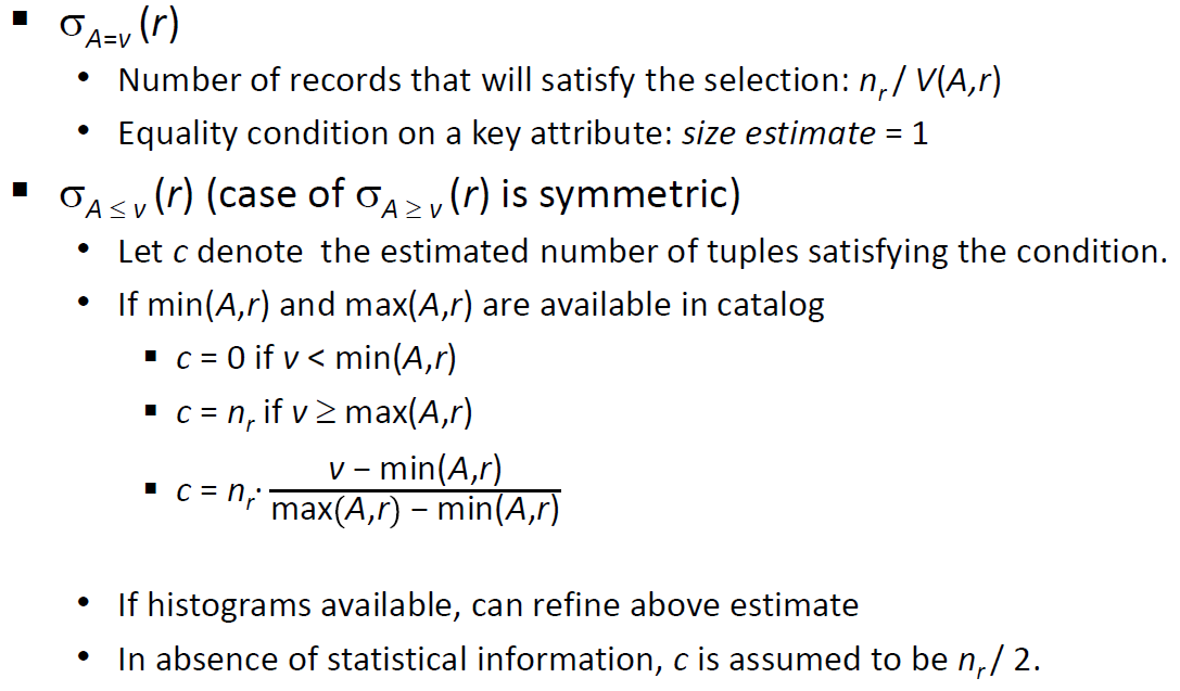
# Statistical Information for Cost Estimation
Important for:
- Can tell how many records to expect
- Can tell performance costs/time
- Selection size estimation
Lecture 4 Query Processing | Lecture 6 Transactions and concurrency