Lecture 4 - Query Processing
# Query Processing
# Basic Steps in Query Processing
- Parsing and translation – Translate the query into its internal form. This is then translated into relational algebra. – Parser checks syntax, verifies relations.
- Optimization – Construct an execution plan that minimizes the cost of query evaluation.
- Evaluation – The evaluation engine takes an execution plan, executes that plan, and returns the answers to the query.
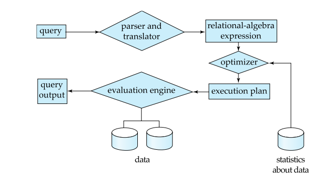
The system’s goal is to create the best execution plan possible.
# Selection Operation
- File/Table scan - algorithms on sequencial data
# Algorithm A1 (linear search, across all records)
Scan each file block and test all records to see whether they satisfy the selection condition. Assumes the data is sequential on disk.
Cost estimate = b_r block transfers + 1 seek
b_r = number of blocks containing records from relation r
Index scan – search algorithms that use an index – selection condition must be on search-key of index.
# A2 (clustered index, equality on key (attr with unique values)).
Usually used when an Index on the PK is setup up Retrieve a single record that satisfies the corresponding equality condition
- Cost = (h_i + 1) * (t_T + t_S)
- h = height of the tree (number of level) of i record
- t_T = block transfer time
- t_S = seek time
# A3 (clustered index, equality on non-key)
Retrieve multiple records.
- Let b = number of blocks containing matching records
- Cost = h_i * (t_T + t_S) + t_S + t_T * b
# A4 (non-clustered index, equality on key/non-key)
Retrieve a single record if the search-key is a candidate key
- Cost = (h_i + 1) * (t_T + t_S) Retrieve multiple records if search-key is not a candidate key
- Cost = (h_i + n) * (t_T + t_S) -> VERY EXPENSIVE AND SLOW
- each of n matching records may be on a different block (TERRIVEL)
- so slow that a full table scan might be faster
- because records are stored in blocks, and in A4 we might be scanning the same block multiple time, as oppose to A1, we only read a block once
It does not matter if an index is clustered or not if you only have to retrieve ONE record. Only one seek time for clustered vs multiple for non-clustered
# Selection Involving Comparisons
Can implement selections in relational algebra. like > or <, by using linear scans or indices:
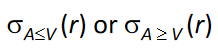
# A5 (clustered index, comparison)
Retrieve multiple records.
- For the first comparison use index to find first tuple >= V and then scan sequentially
- For the second just scan sequentially till first tuple > V; do not use index
# A6 (non-clustered index, comparison)
Retrieve multiple records.
- For first comparison use index to find first index entry >= V and scan index sequentially from there, to find pointers to records
- For second comp. just scan leaf pages of index finding pointers to records, till first entry > V
- In either case, retrieve records that are pointed to
– requires an I/O per record; linear file scan may be cheaper!
# Implementation of Complex Selections
Composite index: index on multiple columns at the same time
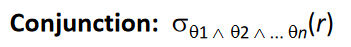
# A7 (conjunctive selection using one index).
Select a combination of selection of columns and algorithms A1 through A7 that results in the
least cost.
Test other conditions on tuple after fetching it into memory
# A8 (conjunctive selection using composite index).
- Use appropriate composite (multiple-key) index if available.
# A9 (conjunctive selection by intersection of identifiers).
Requires indices with record pointers.
Use corresponding index for each condition, and take intersection of all the obtained sets of record pointers.
Then fetch records from file. If some conditions do not have appropriate indices, apply test in memory
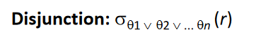
# A10 (disjunctive selection by union of identifiers).
Applicable if all conditions have available indices.
- Otherwise use linear scan.
Use corresponding index for each condition, and take union of all the obtained sets of record pointers.
Then fetch records from file.
- Use linear scan on file
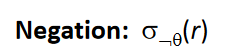
- Or transform the negation O into expression without negation O’, and check if an index is applicable to O’
Find satisfying records using index and fetch from file
# Sorting
Usually we cant bring the whole data into memory to sort it
# External Sort-Merge
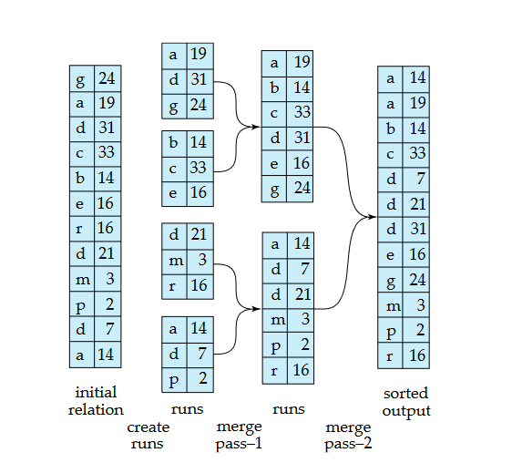
# Steps
- RUNS: Load 3 records, sort, write to disk, repeat
- Now we have multiple temporary files sorted in disk
- MERGE: Pick smallest record from a file and compare it with the records from another file, and write it to another file/disk
- Pick the next smallest record from a file and compare it to the smallest record in another file, output the smallest
- Repeat… and get the sorted output in disk
Allows us to create files larger than out memory Each step has I/O operations. And the number of steps decreases logarithmically with a factor of 2
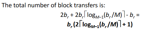
# Cost analysis
The number of blocks in relation r is: b Initial runs I/O: 2b_r block transfers The number of initial runs is: [ b_r /M ] Each merge pass decreases the number of runs by a factor of M-1 The total number of merge passes is: [ log_M–1 (b_r /M) ] Each merge pass reads and writes every block: 2br block transfers For the final pass we don’t count the write cost: -b
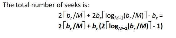
# Cost of seeks:
in the example: 1 seek = 1 block -> 3 records During run generation: one seek to read each run and one seek to write each run : 2[b_r /M ] During the merge phase: Need 2b_r seeks for each merge pass (Except the final one which does not require a write)
# Join Operations
- Several different algorithms to implement joins
- Nested-loop join
- Block nested-loop join
- Indexed nested-loop join
- Merge-join
- Hash-join
- Choice based on cost estimate
# Nested-Loop Join
- 2 Loops:
- Test each record in 1 table against the other
- Unused in EVERY DB system
- Load each record -> load repeated blocks
- Expensive since it examines every pair of tuples in the two relations.
# Block Nested-Loop Join
- Variant of nested-loop join in which every block of inner relation is paired with every block of outer relation:
- 4 Loops
- Loads a block from each table (2 block now in memory)
- Test each record in 1 block against the other block
- We can probably read sequentially from blocks
- Can try all the blocks combinations
- Can be improved with indexes, you dont need to brute force compare all the tuples, nor a full search through the blocks (join on columns for example (ex. NATURAL JOIN))
# Indexed Nested-Loop Join
Index lookups can replace file scans if
- join is an equi-join or natural join and
- an index is available on the inner relation’s join attribute
Can construct an index just to compute a join
4 Loops:
- Full scan on outter loop, but indexed scan in inner loop
# Merge-Join
- Sort both relations on their join attribute (if not already sorted on the join attributes)
- check if record 1 from r matches with record 1 from s
- if yes, output
- if no, step both r and s (a lot of seeks, but we might be able to read multiple blocks into memory)
- repeat…
- “Imagine a zipper”
- Assumes BOTH tables are sorted
- Pointers never go back -> linear complexity
# Hash-Join
- “What if we used the same hash function on both functions?”
- Implies:
- Value X in r goes to Bucket 0
- Same Value X in s goes to Bucket 0
- We only need to compare buckets
- Implies:
- No nested loop, we partition the records in bucket (that fit in memory) and ocmpare them in memory (no disk accesses)
- Hash function can be something like: X mod 5 (no timer)
Cost analysis:
- Partitioning the two relations r and s requires reading and writing every block:
- 2(b_r + b_s)
- Comparing the tuples in the partitions requires reading them once more:
- b_r + b_s
- As a result of the partitioning, there can be some partially filled blocks
- Each partition could have an extra block, and there nh partitions
- These extra blocks must be written (when partitioning) and read (when comparing)
- There are two relations being partitioned
- Therefore, the cost of the hash-join is:
- Block transfers: 3(b_r + b_s) + 4n_h
- Seeks: 2(b_r + b_s) + 2n_h
Because we READ-WRITE-READ, the Hash-Join can be 3x SLOWER than Merge-Join (assuming the tables are sorted). This is the type of decision that the system has to do!
# Blocking Operations
Blocking operations: cannot generate any output until all input is
consumed
e.g., sorting, aggregation, …But can often consume inputs from a pipeline, or produce outputs to a pipeline
Key idea: blocking operations often have two suboperations
– e.g., for sorting: run generation and mergeTreat them as separate operations
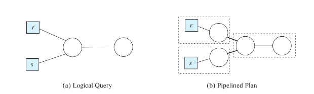
Pipelining: as we generate results, we send them to the next stage
Materialization: we compute the resuts and store them on disk, then read and compute more… (saving in between)
- ex: COUNT operation can be sent as calculated (Pipeline)
- ex: SORTING is a Blocking Operations as we need to save intermediate results (Materialization)